Introduction to Impedance Matching
Impedance matching is a crucial concept in electrical engineering, particularly in the design of radio frequency (RF) and microwave circuits. The primary goal of impedance matching is to maximize power transfer and minimize signal reflections between a source and a load. When the impedance of a source matches the impedance of a load, the maximum amount of power is delivered to the load, and signal reflections are minimized. This is especially important in RF and microwave systems, where impedance mismatches can lead to significant power loss, signal distortion, and reduced overall system performance.
Key Concepts in Impedance Matching
-
Impedance: Impedance is the measure of opposition to the flow of alternating current (AC) in a circuit. It is a complex quantity consisting of both resistance and reactance.
-
Reflection Coefficient: The reflection coefficient (Γ) is a measure of the amount of power reflected from a load due to an impedance mismatch. It is defined as the ratio of the reflected voltage wave to the incident voltage wave.
-
Standing Wave Ratio (SWR): SWR is a measure of the impedance mismatch between a source and a load. It is defined as the ratio of the maximum voltage to the minimum voltage along a transmission line.
-
S-Parameters: Scattering parameters (S-parameters) are used to characterize the behavior of linear electrical networks when undergoing various steady state stimuli by electrical signals.
Impedance Matching Networks
Impedance matching networks are designed to transform the impedance of a load to match the impedance of a source, or vice versa. There are several types of impedance matching networks, each with its own advantages and disadvantages.
Types of Impedance Matching Networks
-
L-Network: An L-network is the simplest type of impedance matching network, consisting of two reactive components (either capacitors or inductors) in an L-shaped configuration.
-
Pi-Network: A Pi-network consists of three reactive components, two shunt components, and one series component, arranged in a π-shaped configuration.
-
T-Network: A T-network consists of three reactive components, two series components, and one shunt component, arranged in a T-shaped configuration.
-
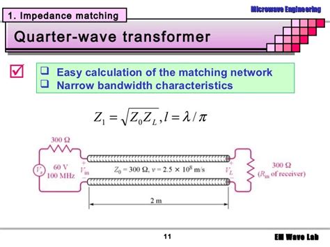
Stub Matching: Stub matching involves using transmission line stubs to match the impedance of a load to a transmission line.
Designing Impedance Matching Networks
When designing an impedance matching network, several factors must be considered, including:
-
Frequency Range: The frequency range over which the impedance matching network must operate.
-
Bandwidth: The bandwidth of the impedance matching network, which determines the range of frequencies over which the network can provide an acceptable match.
-
Component Values: The values of the reactive components used in the impedance matching network must be carefully selected to achieve the desired impedance transformation.
-
Quality Factor (Q): The quality factor of the impedance matching network, which is a measure of the network’s selectivity and loss.
Simulating Impedance Matching Networks
Simulating impedance matching networks is an essential step in the design process, as it allows engineers to predict the performance of the network before building a physical prototype. There are several software tools available for simulating impedance matching networks, including:
-
MATLAB: MATLAB is a high-level programming language and numerical computing environment that can be used to simulate and analyze impedance matching networks.
-
Keysight ADS: Keysight Advanced Design System (ADS) is a powerful electronic design automation software for RF, microwave, and high-speed digital applications.
-
Ansys HFSS: Ansys HFSS is a 3D electromagnetic simulation software for designing and simulating high-frequency electronic products such as antennas, RF/microwave components, and printed circuit boards.
-
Agilent Genesys: Agilent Genesys is an RF and microwave design software that provides a complete set of tools for the design and simulation of impedance matching networks.
Steps in Simulating Impedance Matching Networks
-
Define the Source and Load Impedances: The first step in simulating an impedance matching network is to define the source and load impedances. These impedances can be specified as complex numbers or as S-parameters.
-
Select the Type of Impedance Matching Network: Based on the frequency range, bandwidth, and other design requirements, select the appropriate type of impedance matching network (e.g., L-network, Pi-network, T-network, or stub matching).
-
Design the Impedance Matching Network: Use the selected software tool to design the impedance matching network. This typically involves specifying the component values and the network topology.
-
Simulate the Impedance Matching Network: Once the impedance matching network is designed, simulate its performance using the selected software tool. This typically involves analyzing the network’s S-parameters, reflection coefficient, and SWR over the desired frequency range.
-
Optimize the Impedance Matching Network: Based on the simulation results, optimize the impedance matching network by adjusting the component values and/or network topology to achieve the desired performance.
Analyzing Simulation Results
When analyzing the simulation results of an impedance matching network, several key parameters should be considered:
-
S-Parameters: The S-parameters of the impedance matching network provide a complete characterization of the network’s performance. The most important S-parameters for impedance matching are S11 (input reflection coefficient) and S21 (forward transmission coefficient).
-
Reflection Coefficient: The reflection coefficient (Γ) should be minimized over the desired frequency range to ensure maximum power transfer and minimum signal reflections.
-
SWR: The SWR should be close to 1 over the desired frequency range to indicate a good impedance match between the source and the load.
-
Bandwidth: The bandwidth of the impedance matching network should be sufficient to cover the desired frequency range with acceptable performance.

Example: Simulating an L-Network for Impedance Matching
Let’s consider an example of simulating an L-network for impedance matching using MATLAB.
Problem Statement
Design and simulate an L-network to match a 50 Ω source to a 100 Ω load at a frequency of 1 GHz.
Solution
- Define the Source and Load Impedances:
- Source impedance (Zs) = 50 Ω
-
Load impedance (Zl) = 100 Ω
-
Select the Type of Impedance Matching Network:
-
L-network
-
Design the Impedance Matching Network:
- Calculate the required component values for the L-network using the following equations:
- Q = sqrt((Zl/Zs) – 1)
- C = 1/(2πfQZs)
- L = QZs/(2πf)
-
For this example:
- Q = sqrt((100/50) – 1) = 1
- C = 1/(2π × 1e9 × 1 × 50) = 3.18 pF
- L = 1 × 50/(2π × 1e9) = 7.96 nH
-
Simulate the Impedance Matching Network:
- Use MATLAB to simulate the L-network and analyze its S-parameters, reflection coefficient, and SWR.
MATLAB Code:
% Define source and load impedances
Zs = 50;
Zl = 100;

% Define frequency
f = 1e9;

% Calculate L-network component values
Q = sqrt((Zl/Zs) - 1);
C = 1/(2*pi*f*Q*Zs);
L = Q*Zs/(2*pi*f);

% Create L-network
Lnet = rfckt.matchingnetwork('Topology','L','Frequency',f,'SourceImpedance',Zs,'LoadImpedance',Zl);

% Calculate S-parameters
[s,F] = sparameters(Lnet,{1e9});

% Calculate reflection coefficient and SWR
Gamma = s(1,1);
SWR = (1+abs(Gamma))/(1-abs(Gamma));

% Plot results
figure;
rfplot(Lnet);
title('L-Network Schematic');

figure;
plot(F/1e9,20*log10(abs(s(1,1))),F/1e9,20*log10(abs(s(2,1))));
xlabel('Frequency (GHz)');
ylabel('S-Parameters (dB)');
title('L-Network S-Parameters');
legend('S11','S21');
grid on;

figure;
plot(F/1e9,abs(Gamma));
xlabel('Frequency (GHz)');
ylabel('Reflection Coefficient');
title('L-Network Reflection Coefficient');
grid on;

figure;
plot(F/1e9,SWR);
xlabel('Frequency (GHz)');
ylabel('SWR');
title('L-Network SWR');
grid on;
- Optimize the Impedance Matching Network:
- Based on the simulation results, the L-network provides a good match between the 50 Ω source and the 100 Ω load at 1 GHz.
- If needed, the component values can be further optimized to improve the performance over a specific frequency range.
Simulation Results
The simulation results for the L-network impedance matching example are shown below:
| Parameter | Value at 1 GHz |
|---|---|
| S11 | -30.8 dB |
| S21 | -0.045 dB |
| Γ | 0.0289 |
| SWR | 1.06 |
The simulation results indicate that the L-network provides a good match between the 50 Ω source and the 100 Ω load at 1 GHz, with a low reflection coefficient and an SWR close to 1.
Conclusion
Impedance matching is a critical aspect of RF and microwave circuit design, and simulating impedance matching networks is an essential step in the design process. By using software tools like MATLAB, Keysight ADS, Ansys HFSS, and Agilent Genesys, engineers can design, simulate, and optimize impedance matching networks to achieve maximum power transfer and minimum signal reflections.
When simulating impedance matching networks, it is important to consider factors such as the frequency range, bandwidth, component values, and quality factor. By analyzing the simulation results, including S-parameters, reflection coefficient, and SWR, engineers can determine the performance of the impedance matching network and make necessary adjustments to optimize its performance.
Frequently Asked Questions (FAQ)
-
What is the purpose of impedance matching?
The purpose of impedance matching is to maximize power transfer and minimize signal reflections between a source and a load. When the impedance of a source matches the impedance of a load, the maximum amount of power is delivered to the load, and signal reflections are minimized. -
What are the different types of impedance matching networks?
The main types of impedance matching networks are: - L-network
- Pi-network
- T-network
-
Stub matching
-
What software tools are used for simulating impedance matching networks?
Some popular software tools for simulating impedance matching networks include: - MATLAB
- Keysight ADS
- Ansys HFSS
-
Agilent Genesys
-
What are S-parameters, and why are they important in impedance matching?
S-parameters (scattering parameters) are used to characterize the behavior of linear electrical networks when undergoing various steady state stimuli by electrical signals. In the context of impedance matching, S-parameters provide a complete characterization of the network’s performance, with S11 (input reflection coefficient) and S21 (forward transmission coefficient) being the most important parameters. -
What is the role of the reflection coefficient and SWR in impedance matching?
The reflection coefficient (Γ) is a measure of the amount of power reflected from a load due to an impedance mismatch. It should be minimized over the desired frequency range to ensure maximum power transfer and minimum signal reflections. The standing wave ratio (SWR) is a measure of the impedance mismatch between a source and a load, and it should be close to 1 over the desired frequency range to indicate a good impedance match.
No responses yet